
Bayesian statistics is what all the cool kids are talking about these days. Upon closer inspection, this does not come as a surprise. In contrast to classical statistics, Bayesian inference is principled, coherent, unbiased, and addresses an important question in science: in which of my hypothesis should I believe in, and how strongly, given the collected data?
After briefly stating the fundamental difference between classical and Bayesian statistics, I will introduce three software packages - JAGS, BayesFactor, and JASP - to conduct Bayesian inference. I will analyse simulated data about the effect of wearing a hat on creativity, just as the previous blog post did. In the end I will sketch some benefits a "Bayesian turn" would have on scientific practice in psychology.
Note that this post is very long, introducing plenty of ideas that you might not be familiar with (regrettably, they are not found in the standard university curriculum!). This post should serve as a basic but comprehensive introduction to Bayesian inference for psychologists. Wherever possible, I have linked to additional literature and resources for more in-depth treatments.
After you have read this post, you will begin to understand what the fuss is all about, and you will be familiar with tools to apply Bayesian inference. Let's dive in!
Classical Statistics
What is probability?
Classical statistics conceptualizes probability as relative frequency. For example, the probability of a coin coming up heads is the proportion of heads in an infinite set of coin tosses. This is why classical statistics is sometimes called frequentist. At first glance, this definition seems reasonable. However, to talkabout probability, we now have to think about an infinite repetition of an event (e.g., tossing a coin). Frequentists, therefore, can only assign probability to events that are repeatable. They cannot, for example, talk about the probability of the temperature rising 4 °C in the next 15 years; or Hillary Clinton winning the next U.S. election; or you acing your next exam. Importantly, frequentists cannot assign probabilities to theories and hypotheses - which arguably is what scientists want (see Gigerenzer, 1993).
p values
Because of the above definition of probability, inference in classical statistics is counterintuitive, for students and senior researchers alike (e.g., Haller & Kraus, 2002; Hoekstra, Morey, Rouder, & Wagenmakers, 2014; Oakes, 1986). One notoriously difficult concept is that of the p value: the probability of obtaining a result as extreme as the one observed, or more extreme, given that the null hypothesis is true. To compute p values, we collect data and then assume an infinite repetition of the experiment, yielding more (hypothetical) data. For each repetition we compute a test statistic, such as the mean. The distribution of these means is the sampling distribution of the mean, and if our observed mean is far off in the tails of this distribution, based on an arbitrary standard ($\alpha = .05$) we conclude that our result is statistically significant. For a graphical depiction, see the figure below – inspired by figure 1 in Wagenmakers, 2007.

It is very easy to gloss over these specific assumptions of classical statistics because properties of the sampling distribution are often known analytically. For example, in the case of the t-test, the variance of the sampling distribution is the variance of the actual collected data, divided by the number of data points; $\hat \sigma^2 = \sigma^2 / N$.
Inference based on p values is a remarkable procedure: We assume that we did the experiment an infinite amount of time (we didn't), and we compute probabilities of data we haven't observed, assuming that the null hypothesis is true. This way of drawing inferences has serious deficits. For an enlightening yet easy to read paper about these issues, see Wagenmakers (2007). If you think that you could need a more detailed refresher on p values - they are tricky! - see here.
Confidence Intervals
Recently, the (old) new statistics has been proposed, abandoning p values and instead focusing on parameter estimation and confidence intervals (Cumming, 2014). As we will see later, parameter estimation and hypothesis testing answer different questions, so abandoning one in favour of the other is misguided. Because confidence intervals are still based on classical theory, they are an equally flawed method of drawing inferences; see Lee (n.d.) and Morey et al. (submitted).
What are parameters?
Tied to the classical notion of probability, classical statistics considers the population parameter as fixed, while the data are allowed to vary (repeated sampling). For example, the difference between men and women in height is exactly 15 centimeters. We can intuit that confidence intervals, as well as statistical power, are not concerned with the actual data we have collected. Why?
Assume we collect height data from men and women, and compute a 95% confidence interval around our difference estimate - this does not mean that we are 95% confident that the true parameter lies within these bounds! For the actual experiment, the true parameter either is or is not within these bounds. 95% confidence intervals state that, if we were to repeat our experiment an infinite amount of time, in 95% of all cases the parameter will be within those bounds (Hoekstra, Morey, Rouder, & Wagenmakers, 2014). This must be so because we can only talk about probability as relative frequency: we have to assume repeating our experiment, even though we only conducted one!
It is important to note that all probability statements in classical statistics are of that nature: they average over an infinite repetition of experiments. Probability statements do not pertain to the specific data you gathered; they are about the testing procedure itself. Extend this to statistical power, which is the probability of finding an effect when there really is one. High-powered experiments yield informative data, on average. Low-powered experiments yield uninformative data, on average. However, for the specific experiment actually carried out - once the data are in - we can go beyond power as a measure of how informative our experiment was (Wagenmakers et al., 2014). In the last section I explain what this entails when using Bayesian inference for hypothesis testing.
Bayesian Statistics
What is probability?
In Bayesian inference, probability is a means to quantify uncertainty. Continuing with the height example above, Bayesians quantify uncertainty about the difference in height with a probability distribution. It might be reasonable, for example, to specify a normal distribution with mean $\mu = 15$ and variance $\sigma^2 = 4$
\begin{equation*}
\text{difference} \sim \mathcal{N}(15, 4)
\end{equation*}
We most strongly believe that the height difference is 15 centimeters, although it could also be 10, or even 5 centimeters (but with lower probability). However, we might not be so sure about our estimates. To incorporate uncertainty, we could increase the variance of the distribution (decrease the "peakedness"), say, in this case, to $\sigma^2 = 16$. The plot below compares possible prior beliefs (click on the image to enlarge it).

In the Bayesian world, probability retains the intuitive, common-sense interpretation: it is simply a measure of uncertainty.
What are parameters?
While parameters still have one single true value in some ontological sense, men are on average exactly 15 centimeters taller than women, we quantify our uncertainty about this difference with a probability distribution. The beautiful part is that, if we collect data, we simply update our prior beliefs with the information that is in the data to yield posterior beliefs.
Bayesian Parameter Estimation
There's no theorem like Bayes' theorem
Like no theorem we know
Everything about it is appealing
Everything about it is a wow
Let out all that a priori feeling
You've been concealing right up to now!
- George Box
Because parameters themselves are assigned a distribution, statistical inference reduces to applying the rules of probability. We specify a joint distribution over data and parameters, $p(\textbf{y}, \theta)$. By the definition of conditional probability we can write $p(\textbf{y}, \theta) = p(\textbf{y}|\theta)p(\theta)$. The first term, $p(\textbf{y}|\theta)$, is the likelihood, and it embodies our statistical model. It also exists in the frequentist world, and it contains assumptions about how our data points are distributed; for example, whether they are normally distributed or Bernoulli distributed. The other term, $p(\theta)$, is called the prior distribution over the parameters, and quantifies our belief (before looking at data) in, say, height differences among the sexes.
Combining the data we have collected with our prior beliefs is done via Bayes' theorem:
\begin{equation*}
p(\theta|\textbf{y}) = \frac{p(\theta) \times p(\textbf{y}|\theta)}{p(\textbf{y})}
\end{equation*}
where $\textbf{y}$ is the probability of the data (which has no frequentist equivalent); in words:
\begin{equation*}
\text{posterior} = \frac{\text{prior} \times \text{likelihood}}{\text{marginal likelihood}}
\end{equation*}
Because $p(\textbf{y})$ is just a normalizing constant so that $p(\theta|\textbf{y})$ sums to 1, i.e. is a proper probability distribution, we can drop it and write:
\begin{equation*}
p(\theta|\textbf{y}) \sim p(\theta) \times p(\textbf{y}|\theta)
\end{equation*}
With Bayes' rule we are solving the "inverse probability problem", that is we are going from the effect (the data) back to the cause (the parameter) (Bayes, 1763; Laplace 1774).
Classical statistics has a whole variety of estimators, such as maximum likelihood and generalized least squares, which are investigated along specific dimensions (e.g. bias, efficiency, consistency). In contrast, Bayesians always uses Bayes' rule, which simply follows from probability. This is why we say that Bayesian statistics is principled, rational, and coherent. Let's take a look at a simple example to see how the two estimation approaches differ.
A simple example
Suppose you flip a coin twice and observe heads both times. What is your estimate that the next coin flip comes up heads? We know that flipping a coin several times, with the flips being independent, can be described binomially with likelihood:
\begin{equation*}
L(\theta| \textbf{y}) = \theta^k \times (1 - \theta)^{N - k}
\end{equation*}
where $N$ is the number of flips and $k$ is the number of heads. The likelihood $L(\theta| \textbf{y})$ is just the probability expressed in terms of the parameter $\theta$, instead of the data $\textbf{y}$ (and need not sum to 1). For example, assuming $\theta = .5$, the likelihood is:
\begin{align*}
L(\theta = .5 | \textbf{y}) &= .5^2 \times (1 - .5)^{2-2} \\
L(\theta = .5 | \textbf{y}) &= .25
\end{align*}
Plotting the likelihood for the whole range of possible $\theta$ values given our data ($k = 2$ and $N = 2$) yields:
curve(dbinom(2, 2, prob = x), from = 0, to = 1, ylab = 'likelihood')

We see that $\theta = 1$ maximizes the likelihood; in other words: $\theta = 1$ is the maximum likelihood estimator (MLE) for these data. Maximum likelihood estimation is the workhorse of classical inference. In classical statistics, then, the prediction for the next coin coming up heads would be 1. This is somewhat counterintuitive; would that really be your prediction, after just two coin flips? What does the Bayesian in you think?
First, we need to quantify our prior belief about the parameter $\theta$. Invoking the principle of insufficient reason, we use a prior that assigns equal probability to all possible values of $\theta$: the uniform distribution. We can write this as a Beta distribution with parameters $a = 1, b = 1$:
\begin{equation*}
\mathrm{Beta}(\theta|a, b) = \textbf{K} \times \theta^{a - 1} (1 - \theta)^{b - 1}
\end{equation*}
where $\textbf{K}$ is the normalizing constant and not of importance for now. $a$ and $b$ can be interpreted as prior data. In our example, $a$ would be the number of heads and $b$ would be the number of tails. Remember that in Bayesian inference we just multiply the likelihood with the prior. The Beta distribution is a conjugate prior for the binomial likelihood. This means that when using this prior, the posterior will again be a Beta distribution, making for trivial computation. Plugging in Bayes' rule yields:
\begin{align*}
p(\theta|N, k) &\sim \theta^k (1 - \theta)^{N - k} \times \theta^{a - 1} (1 - \theta)^{b - 1} \\
p(\theta|2, 2) &\sim \theta^2 (1 - \theta)^{2 - 2} \times \theta^{a - 1} (1 - \theta)^{b - 1} \\
p(\theta|2, 2) &\sim \theta^{a - 1 + 2} (1 - \theta)^{b - 1 + 2 - 2}
\end{align*}
Rearranging yields:
\begin{equation*}
p(\theta|2, 2) \sim \theta^{(a + 2) - 1} (1 - \theta)^{(b + 2 - 2) - 1}
\end{equation*}
We recognize that our posterior is again a Beta distribution: it's Beta(3, 1). In general, our updating rule is $Beta(a + k, b + N - k)$.

The point with the most probability density, the mode, is $(a - 1) / (a + b - 2)$ which in our case yields $1$. However, as we see when looking at the distribution, there is substantial uncertainty. To account for this, we take the mean of the posterior distribution, $a / (a + b)$, as our best guess for the future. Thus, the prediction for the next coin flip being heads is $.75$. Note that classical estimation, based on maximum likelihood ($\theta_{MLE} = k / N = 2 / 2$), would predict heads with 100% certainty. For more on likelihoods, check out this nice blog post. For more details on Bayesian updating, see this.
What can be seen in conjugate examples quite clearly is that the Bayesian posterior is a weighted combination of the prior and the likelihood. We have seen that the posterior mean is:
\begin{equation*}
\hat p = \frac{k + a}{a + b + n}
\end{equation*}
which, with some clever rearranging, yields:
\begin{equation*}
\hat p = \frac{n}{a + b + n}(\frac{k}{n}) + \frac{a + b}{a + b + n}(\frac{a}{a + b})
\end{equation*}
Both the maximum likelihood estimator $\theta_{MLE} = k / n$ and the mean of the prior $a / (a + b)$ are weighted by terms that depend on the sample size $n$ and the prior parameters $a$ and $b$. Two important things should be noted here. First, this implies that the posterior mean is shrunk toward the prior mean. In hierarchical modeling, this is an extremely powerful idea. Shrinkage yields a better estimator (Efron & Morris, 1977). For a nice tutorial on hierarchical Bayesian inference, see Sorensen & Vasishth (submitted).
The second thing to note is that when $n$ becomes very large, the Bayes point estimate and the classical maximum likelihood estimate converge to the same value (Bernstein-von Mises theorem). You can see this in the formula above. The first weight becomes 1 and the second weight becomes 0, leaving only $k / n$, which is the maximum likelihood estimate. Therefore, when different people initially disagree (different prior), once they have seen enough evidence, they will agree (same posterior).
Note that identical estimation results need not lead to the same model comparison results. I find the argument that because the estimation converges, we can just go on doing frequentist statistics rather disturbing. First, you never have an infinite amount of participants. Second, the prior allows you to incorporate theoretical meaningful information into your model, which can be extremely valuable (e.g. this great problem). Third, and most important, estimation and testing answer different questions. While parameter estimates might converge, Bayesian hypothesis testing offers a much more elegant and richer inferential foundation over that provided by classical testing (but more on this below).
Markov chain Monte Carlo
Using a simple example, we have seen how Bayesians update their prior beliefs upon seeing new data, yielding posterior beliefs. However, conjugacy is not always given, and the prior times the likelihood might be a unusually formed, complex distribution that we cannot track analytically. For most of the 20th century, Bayesian analysis was restricted to conjugate priors for computational simplicity.
But things have changed. Due to the advent of cheap computing power and Markov chain Monte Carlo techniques (MCMC) we now can estimate basically every posterior distribution we like.
Bayesian hypothesis testing
Parameter estimation is not the same as testing hypotheses (e.g. Morey, Rouder, Verhagen, & Wagenmakers, 2014; Wagenmakers, Lee, Rouder, & Morey, submitted). The argument is simple: while each observation tells you something about the parameter, not every observation is informative about which hypothesis you should believe in. To build an intuition for that, let's throw a coin (again). Is it a fair coin ($\theta = .5$) or a biased ($\theta \neq .5$) coin? Assume the first observation is heads. You learn something about the parameter $p$; for example, it can't be equal to 0 (always tails), and that a bias toward heads is more likely than a bias toward tails. Looking only at the parameter estimate thus carries some evidence against the null hypothesis. However, in fact you have learned nothing that would strengthen your belief in either of your hypotheses. Observing heads is equally consistent with the coin being unbiased and the coin being biased (the Bayes factor is equal to 1, but more below). Inference by parameter estimation is inadequate, unprincipled, and biased.
In order to test hypotheses, we have to compute the marginal likelihood, which we can skip when doing parameter estimation (because it is just a constant). As a reminder, here is the formula again:
\begin{equation*}
\text{posterior} = \frac{\text{prior} \times \text{likelihood}}{\text{marginal likelihood}}
\end{equation*}
Let's say we compare two models, $M_0$ and $M_1$, that describe a difference in the creativity of people who wear hats and others who don't. The parameter of interest is $\delta$. $M_0$ restricts $\delta$ to 0, while $M_1$ lets $\delta$ vary. This corresponds to testing a null hypothesis $H_0: \delta = 0$ against the alternative $H_1: \delta \neq 0$. In order to test which hypothesis is more likely to be true, we pit the predictions of the models against each other. The prediction of the models is embodied by their respective marginal likelihoods, $p(\textbf{y}|M)$. For the discrete case, this yields:
\begin{equation*}
P(\textbf{y}|M) = \sum_{i=1}^{k} P(\textbf{y}|\theta_i, M)P(\theta_i|M)
\end{equation*}
That is, we look at the likelihood of the data $\textbf{y}$ for every possible value of $\theta$ and weight these values with our prior belief. For continuous distributions, we have an integral:
\begin{equation*}
p(\textbf{y}|M) = \int_{}^{} p(\textbf{y}|\theta, M)p(\theta|M)d\theta
\end{equation*}
The ratio of the marginal likelihoods is the Bayes factor (Kass & Raftery, 1995):
\begin{equation*}
BF_{01} = \frac{p(\textbf{y}|M_0)}{p(\textbf{y}|M_1)}
\end{equation*}
which is the factor by which our prior beliefs about the hypotheses (not parameters!) get updated to yield the posterior beliefs about which hypothesis is more likely:
\begin{equation*}
\frac{p(M_0|\textbf{y})}{p(M_1|\textbf{y})} = \frac{p(\textbf{y}|M_0)}{p(\textbf{y}|M_1)} \frac{p(M_0)}{p(M_1)}
\end{equation*}
The Bayes factor is a continuous measure of evidence: $BF_{01} = 3$ indicates that the data are three times more likely under the null model $M_0$ than under the alternative model $M_1$. Note that $BF_{10} = 1 / BF_{01}$, and that when the prior odds are 1, the posterior odds equal the Bayes factor.
Because complex models can capture many different observations, their prior on parameters $p(\theta)$ is spread out wider than those of simpler models. Thus there is little density at any specific point - because complex models can capture so many data points; taken individually, each data point is comparatively less likely. For the marginal likelihood, this means that the likelihood gets multiplied with these low density values of the prior, which decreases the overall marginal likelihood. Thus model comparison via Bayes factors incorporates an automatic Ockham's razor, guarding us against overfitting.
While classical approaches like the AIC naively add a penalty term (2 times the number of parameters) to incorporate model complexity, Bayes factors offer a more natural and principled approach to this problem. For details, see Vandekerckhove, Matzke, & Wagenmakers (2014).
Two priors
Note that there are actually two priors – one over models, as specified by the prior odds $p(M_0) / p(M_1)$, and one over the parameters, $p(\theta)$, which is implicit in the marginal likelihoods. The prior odds are just a measure of how likely one model or hypothesis is over the other, prior to data collection. It is irrelevant for the experiment at hand, but might be important for drawing conclusions. For example, Daryl Bem found a high Bayes factor in support of precognition. Surely this does not by itself mean that we should believe in precognition! The prior odds for pre-cognition are extremely low - at least for me - so that even if multiplied by a Bayes factor of 1000, the posterior odds will be vanishingly small:
\begin{equation*}
\frac{1}{100000} = \frac{1000}{1} \cdot \frac{1}{100000000}
\end{equation*}
We can agree on how much the data support precognition (as quantified by the Bayes factor). However, this does not mean we have to buy it. Extraordinary claims require extraordinary evidence.
Savage-Dickey trick
For the univariable case, computing the marginal likelihood is pretty straightforward; however, the integrals get harder with many variables, say in multiple regression. Note that while parameter estimation is basically solved with MCMC methods, computing the marginal likelihood is still a tough deal. However, when testing nested models, such as in the case of null hypotheses testing, we can use a neat mathematical trick that sidesteps the issue of computing the marginal likelihood – the Savage-Dickey density ratio:
\begin{equation*}
BF_{01} = \frac{p(\delta = 0|M_1, \textbf{y})}{p(\delta = 0|M_1)}
\end{equation*}
That is, take the ratio of the posterior density at the point of interest, for example $\delta = 0$, and divide it by the prior density at the point of interest. Note that unlike to the p value, the Bayes factor is not limited to testing nested models, but can compare complex, functionally different models (as is common in cognitive science). We will see a nice graphical depiction of Savage-Dickey later.
Let us revisit our coin toss example. We flipped the coin twice and observed heads both times. Suppose we want to test the hypothesis that the coin is fair – that is $\theta = .5$. Using the Savage-Dickey density ratio, we divide the height of the posterior distribution at $\theta = .5$ by the height of the prior distribution at $\theta = .5$. Recall that:
\begin{align*}
p(\theta) \sim \text{Beta(1, 1)} \\
p(\theta|\textbf{y}) \sim \text{Beta(3, 1)} \\
\end{align*}
Thus yielding:
\begin{align*}
BF_{01} &= \frac{p(\theta = .5|\textbf{y})}{p(\theta = .5)} \\
BF_{01} &= \frac{.75}{1} \\
BF_{10} &= 1\frac{1}{3} \\
\end{align*}
The data are $1\frac{1}{3}$ times more likely under the model that assumes that the coin is biased toward either heads or tails. For a nice first lesson in Bayesian inference that prominently features coin tosses with interactive examples, see this. For an excellent introduction to the Savage-Dickey density ratio, see Wagenmakers et al. (2010).
Lindley's paradox and the problem with uninformative priors
Uninformative priors like $\text{Unif(}-\infty\text{,}+\infty\text{)}$ can be used in parameter estimation because the data quickly overwhelm the prior. However, when testing hypotheses, we need to use priors that are at least somewhat informative. One can see the problem with uninformative priors in the Savage-Dickey equation. These priors spread out their probability mass such that at each point there is virtually zero density. Dividing something by a very, very small number yields a very, very high number. The resulting Bayes factor favours the null hypothesis without bounds (DeGroot, 1982; Lindley, 1957). Consequently, we need to use informative priors for hypothesis testing. Rouder, Morey, Wagenmakers and colleagues have extended the default priors initially proposed by Harold Jeffreys (1961). These default priors have certain important features, see Rouder & Morey (2012), but should be given some thought and possible adjustments before used.
Creativity example
We want to know if wearing hats does indeed have an effect on creativity. Instead of collecting real data, we just simulate data, assuming a real effect of Cohen's $d = 7 / 15$.
set.seed(666)

x <- rep(0:1, each = 50)
y1 <- rnorm(50, mean = 50, sd = 15)
y2 <- rnorm(50, mean = 57, sd = 15)
dat <- data.frame(y = c(y1, y2), x = x)

boxplot(y ~ x, dat, col = c('blue', 'green'),
        xlab = 'condition', ylab = 'creativity')

Classical Inference
In classical statistics we would compute p values. Because the t-test is simply a general linear model with one categorical predictor, we can run:
summary(lm(y ~ x, dat))

## Call:
## lm(formula = y ~ x, data = dat)
##
## Residuals:
##     Min      1Q   Median     3Q     Max
## -43.120 -10.578   0.219  11.295  33.223
##
## Coefficients:
##             Estimate Std. Error t value Pr(>|t|)
## (Intercept)   49.028   2.195     22.339
If you are not familiar with R, this output might look daunting. Note that the t-test as a general linear model states that
\begin{equation*}
y_i = \beta_0 + \beta_1 x_i + \epsilon_i
\end{equation*}
In the R output, (Intercept) is $\beta_0$, while x is $\beta_1$. $\beta_0$ is the mean of the group in which our categorical predictor is 0, i.e. the group which did not wear hats. The group that did wear hats, on the other hand, gets a creativity boost of 6.944. The p value for this difference is $p = .028$. We would conclude that the probability of observing these data or more extreme data given that there really is no effect is only 2.8%. Using the conventional cutoff, $\alpha = .05$, we would say our result is statistically significant. Although we have not computed $p(H_1|\textbf{y})$, we would conclude that the result supports the alternative hypothesis. Is this really so?
Bayesian Inference
Below I introduce three sofware packages for Bayesian inference. The first one, JAGS, is very low-level and does not readily provide Bayes factors. Its primary use is to estimate the posterior distribution. In our present example, we are interested in the difference between the two groups, specifically in the effect size. As mentioned earlier, we can use uninformative priors for parameter estimation. To get a feeling for slightly informative priors, however, I will specify default priors when using JAGS. Subsequently we will compute Bayes factors using the BayesFactor R package and the graphical software JASP.
Using JAGS
JAGS ("Just Another Gibbs Sampler") implements MCMC methods (as discussed above) to sample from the posterior distribution. This is especially needed when the posterior distribution is not available in closed form - say when we don't have conjugate priors.
To have a scale-free measure of our prior belief, we will specify our prior beliefs over the effect size $\delta = \mu / \sigma^2$. As suggested in the literature, we might want to use a default prior. For a detailed rationale of so-called default priors, see pages 6 and 7 of this, Rouder, Speckman, Sun, Morey, & Iverson (2009), and Rouder & Morey (2012). For a more thorough treatment of the default prior approach pioneered by Harold Jeffreys, see Ly et al. (in press).
Constructing a default prior
What is our prior on the effect size? We might want to use a normal distribution centered on 0:
\begin{equation*}
\delta \sim \text{Normal(0, g)}
\end{equation*}
The more difficult question is how to specify the variance, $g$. If we specify large values, then we say that we also expect very high values for the effect size, like 2 or 3. This never happens in psychology! Perhaps we should choose a lower value, like 1? Or better yet, why not quantify our uncertainty about the variance with ... a probability distribution!
This is what we will do, using the inverse Gamma distribution which has two parameters:
\begin{equation*}
g \sim \text{Inverse Gamma(}\frac{1}{2}\text{,}\frac{r^2}{2}\text{)}
\end{equation*}
Now when we integrate out the parameter $g$, that is incorporate our uncertainty about the variance in our belief about the effect size, this elaborate prior specification simplifies to:
\begin{equation*}
\delta \sim \text{Cauchy(r)}
\end{equation*}
The Cauchy distribution has only one parameter, $r$. It is similar to a normal distribution, but with fatter tails (indicating greater uncertainty). The scale parameter $r$ influences the width of the distribution; the higher the parameter value, the wider the distribution – meaning greater probability density at the tails.
Are we done? Not quite! We still need to specify a prior over the variance. Because we do not make inference about the variance, we can give it a noninformative, Jeffreys' prior. We approximate the Jeffreys' prior using an inverse Gamma distribution with very small shape and rate parameters (e.g. Morey, Rouder, Pratte, & Speckman, 2011):
\begin{equation*}
\sigma^2 \sim \text{Inverse Gamma(.00001, .00001)}
\end{equation*}
We also have to specify a prior distribution over $\beta_0$, the mean of the group that did not wear hats. Again, because our inference does not depend on this parameter, we assign it an uninformative prior:
\begin{equation*}
\beta_0 \sim \text{Normal(0, 10000)}
\end{equation*}
Note that the specification in JAGS does not use the variance $\sigma$, but precision, which is $1 / \sigma$. Therefore, to specify a high variance, we would use a low precision.
Although it is possible to compute Bayes factors directly in JAGS, for example using the product-space method (Lodewyckx et al., 2011) or conditional marginal density estimation (Morey et al., 2011), it is primarily used to estimate posterior distributions of parameters of interest. In the example that follows, we will compute Bayes factors with easier-to-use software and use JAGS to estimate posterior distributions. By the way, if you are lost with all those different distributions, check out Richard Morey's nice interactive visualisations.
Note that the general linear model assumes that:
\begin{equation*}
y_i = \beta_0 + \beta_1 x_i + \epsilon_i
\end{equation*}
\begin{equation*}
\epsilon \sim \text{Normal(}0, \sigma)
\end{equation*}
that is the errors are normally distributed and centered at 0. From this it follows that:
\begin{align*}
y_i \, - (\beta_0 + \beta_1 x_i) &\sim \text{Normal(}0, \sigma) \\
y_i &\sim \text{Normal(}\beta_0 + \beta_1 x_i, \sigma)
\end{align*}
which is the specification used in JAGS (with precision instead of variance).
library('rjags') # for communicating with JAGS
library('ggmcmc') # for nice visualizations
options(scipen = 100, digits = 5)

model_string <- '
model {
  ### priors
  sigma ~ dgamma(.00001, .00001)          # [Jeffreys prior]
  d ~ dnorm(0, invg)                      # [prior on effect size d]
  invg ~ dgamma(1/2, rsqr/2)              # [prior on variance of d]
  b0 ~ dnorm(0, .0001)                    # [mean of the non-hat group]
  tau <- pow(sigma, -2)                   # [precision = 1/variance]
  b1 <- d * sigma                         # [difference between non-hat & hat]

  ### likelihood
  for (i in 1:N) {
    y[i] ~ dnorm(mu[i], tau)
    mu[i] <- b0 + b1 * x[i] # [t-test as a general linear model]
  }
}'

params <- c('b0', 'b1', 'd')
data <- list('x' = dat$x, 'y' = dat$y, 'rsqr' = sqrt(2)/2, 'N' = nrow(dat))
model <- jags.model(textConnection(model_string), data = data, n.chains = 3)
samples <- coda.samples(model, n.iter = 100000, variable.names = params)
The plot below shows the posterior distributions of b0 (the mean in the no-hats condition), b1 (the difference between the two groups), and d (effect size):
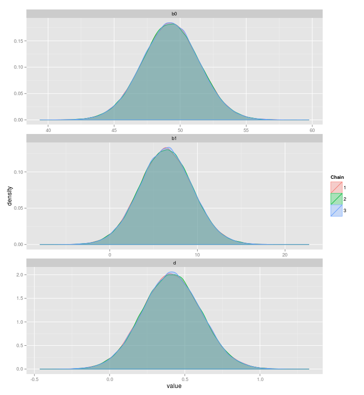
How wonderful! Instead of a point estimate, we get a whole distribution. It is important to check if the MCMC algorithm actually converged on the posterior distribution. Run the commands below to monitor convergence:
#samp <- ggs(samples)
#ggs_autocorrelation(samp)
#ggs_traceplot(samp)
#ggs_geweke(samp)
#ggs_Rhat(samp)
#ggs_running(samp)
Upon inspection, everything seems fine!
Let's compute credibility intervals – the Bayesian analogue to confidence intervals:
HPDinterval(samples)[[1]]

##       lower    upper
## b0 44.846982 53.24459
## b1  0.362848 12.15736
## d   0.034575  0.80231
## attr(,"Probability")
## [1] 0.95
We can be 95% confident that the effect size is between .034 and .802. There is substantial variability, but that's just how things are (also this). Note that, in this case, the frequentist confidence interval coincides with the Bayesian credibility interval.
What John Kruschke and other advocates of "Hypothesis testing via Estimation" would have us look at to draw inferences is only these posterior distributions. Simplifying a bit, if the 95% credibility interval of d excludes 0 (or some specified region of interest, say -.1 to .1), we would conclude that there really is an effect. As I have said in the section introducing the Bayes factor, this is a little fishy. It is unprincipled – how strongly should we believe in an effect? And it is biased against $H_0$ – we will see below that there is not much evidence for an effect.
Note that we might have outliers in our data, rendering the normal distribution inadequate. Thanks to JAGS's flexibility, we can easily substitute the normal distribution with a t-distribution, which has fatter tails. This would make our inference more robust, see e.g. chapter 16 in Kruschke (2014).
Concluding the section on JAGS, I want to say that JAGS offers a lot of flexibility, but at the price of complexity. Below I introduce you to more user-friendly software, which also enables us to easily compute Bayes factors for common designs. However, if you are doing multivariate statistics like structural equation modeling, there is no way around software like JAGS. If you are interested in cognitive modeling of the Bayesian kind, you also need to use JAGS. For a great book on Bayesian cognitive modeling, see Lee & Wagenmakers (2013).
Using BayesFactor
The BayesFactor R package written by Richard Morey computes the Bayes factor for a variety of common statistical models. Similarly to the frequentist analysis above, we specify the t-test as a general linear model and use the function lmBF from the BayesFactor package:
library('BayesFactor')

lmBF(y ~ x, dat)

## Bayes factor analysis
## --------------
## [1] x : 1.8934 ±0%
## Against denominator:
## Intercept only
## ---
## Bayes factor type: BFlinearModel, JZS
The resulting Bayes factor is $BF_{10} = 1.84$, that is the model that assumes an effect of hat is 1.84 times more likely then the model that assumes no effect – given a so-called JZS prior specification. JZS stands for Jeffreys-Zellner-Siow. This prior is basically the same we have specified before. For a more detailed rationale, see Rouder et al. (2009).
The BayesFactor package also does ANOVA, multiple regression, proportions and more - do have a look! For a more detailed explanation of the Bayesian t-test, see this. For a tutorial on regression that uses the BayesFactor package, click here.
Using JASP
"Gosh!" You might say. "This looks all very peculiar. I am not familiar with R, let alone with JAGS. Bayes seems complicated enough. Oh, I better stick with p values and SPSS."
NOOOOOOOOOOOOOOOOOOOOOOOOOO. There is a better way!
JASP is a slick alternative to SPSS that also provides Bayesian inference (and it does APA tables!). First, let us write the data to a .csv file:
write.csv(dat, file = 'creativity.csv', row.names = FALSE)
Open JASP, read in the .csv file, and run a Bayesian independent t-test. Checking Prior and Posterior and Additional Info gives us a beautiful plot summarizing the result:

Above you can see the Savage-Dickey density ratio, i.e. the height of the posterior divided by the height of the prior, at the point of interest (here $\delta = 0$).
Is this result consistent for different prior specifications? Checking Bayes factor robustness check yields the following result:

We see that across different widths (0-1.5) of the Cauchy prior, the conclusion roughly stays the same. If we were to specify a width of 200, what would happen? Lindley would turn around in his grave! As mentioned above in the section on Lindley's paradox, uninformative priors should not be used for hypothesis testing because this leads the Bayes factor to strongly support $H_0$. You can see that in the graph below.

Setting aside unreasonable prior specifications, the Bayes factor is not very different from 1. This means that our data are not sufficiently informative to choose between the hypotheses. While the Bayes factor is a continuous measure, it might be reasonable to label certain categories depending on the magnitude of the Bayes factor. Several labels have been proposed. For an overview, see this. To get some intuition how a Bayes factor "feels", see here.
Because the data are not compelling enough, we run an additional 20 participants per group:
set.seed(1000)
x <- rep(0:1, each = 20)
y1.2 <- rnorm(20, mean = 50, sd = 15)
y2.2 <- rnorm(20, mean = 57, sd = 15)
dat.2 <- data.frame(y = c(y1.2, y2.2), x = x)
dat.both <- rbind(dat, dat.2)
A quick look tells us that the Bayes factor in favour of the alternative hypothesis is now roughly 25:
lmBF(y ~ x, dat.both)

## Bayes factor analysis
## --------------
## [1] x : 24.94 ±0%
## Against denominator:
## Intercept only
## ---
## Bayes factor type: BFlinearModel, JZS
We can see how the Bayes factor develops over the data collection using JASP. First, let's write the data to disk again:
write.csv(dat.both, file = 'creativity.csv', row.names = FALSE)
Running the same analysis in JASP in order to get those stunning graphs yields:

Checking Sequential Analysis yields:

This plot shows how the Bayes factor develops over the course of participant collection.
JASP includes several interesting datasets. I encourage you to play with them! Peter Edelsbrunner and I recently gave a workshop where we had some exercises and more datasets. You can find the materials here.
Advantages of Bayesian inference
The right kind of probability
I don't think that researchers are really interested in the probability of the data (or more extreme data), given that the null hypothesis is true and the data was collected according to a specific (unknown) sampling plan. Rather, I believe that scientists care about which hypothesis is more likely to be true after the experiment has been conducted. In the same vein, we don't care about how often, in an infinite repetition of the experiment, the parameter estimate lies in a specific interval. We prefer a statement of confidence. How confident can I be that the parameter estimate lies in this specific interval?
"Subjectivity"
"Today one wonders how it is possible that orthodox logic continues to be taught in some places year after year and praised as 'objective', while Bayesians are charged with 'subjectivity'. Orthodoxians, preoccupied with fantasies about nonexistent data sets and, in principle, unobservable limiting frequencies – while ignoring relevant prior information – are in no position to charge anybody with 'subjectivity'."
- Jaynes (2003, p. 550), as cited in Lee & Wagenmakers (2014, p. 61)
Bayesian inference conditions only on the observed data, that is it does not violate the likelihood principle, and so is independent of the researcher's intentions. This might sound surprising, but p values are inherently subjective – in a really nasty way. For theoretical arguments about that, see Berger & Berry (1988) and Wagenmakers (2007). Scientific objectivity is illusionary, and both frequentist and Bayesian methods have their subjective elements. Crucially, though, Bayesian subjectivity is open to inspection by everyone (just look at the prior!), whereas frequentist subjectivity is not.
Optional Stopping
"The rules governing when data collection stops are irrelevant to data interpretation. It is entirely appropriate to collect data until a point has been proven or disproven, or until the data collector runs out of time, money, or patience."
- Edwards, Lindman, & Savage (1963, p. 239)
Bayesians do not have an optional stopping problem (Edwards et al., 1963; Rouder, 2014). Recall that in classical statistics, you cannot collect additional data once you have run your test, because this inflates the nominal $\alpha$ level; that is it will rain false positives (Simmons, Nelson, & Simonsohn, 2011). For example, let's say you test 20 participants and get $p = .06$. You cannot test another batch of, say 5, and run your test again. In a sense, you are in limbo. You can neither conclude that $H_1$ is supported, nor that $H_0$ is supported, nor that the data are uninformative. On other occasions you might want to stop early because the data show a clear picture, and running more subjects might be expensive or unethical. However, within the framework of classical statistics, you are not permitted to do so. Using Bayesian inference, we can monitor the evidence as it comes in, that is test after every participant, and stop data collection once the data are informative enough – say the Bayes factor in favour of $H_0$ or $H_1$ is greater than 10. For a recent paper on sequential hypothesis testing, see Schönbrodt (submitted).
Continuous Measure of Evidence
The Bayes factor is a continuous measure of evidence and is directly interpretable. While inference in current statistical practices relies on an arbitrary cutoff of $\alpha = .05$ and results in a counterfactual (probability of at least as extreme data, given $H_0$), Bayes factors straightforwardly tell you which hypothesis is more likely given the data at hand.
Supporting the null
Bayes factors explicitly look at how likely the data are under $H_0$ and $H_1$. Recall that the p value looks at the probability of the data (or more extreme data), given that $H_0$ is true. The logic behind inference, called Fisher's disjunction, is as follows: either a rare event has occured (with probability $p$), or $H_0$ is false. In the form of a syllogism, we have:
(Premise) If $H_0$, then y is very unlikely.
(Premise) y.
(Conclusion) $H_0$ is very unlikely.
This reasoning is flawed, as demonstrated by the following:
(Premise) If an individual is a man, he is unlikely to be the Pope.
(Premise) Francis is the Pope.
(Conclusion) Francis is probably not a man.
Nonsense! The problem is that in classical inference, we do not look at the probability of the data under $H_1$. The data at hand, Francis being the Pope, are infinitely more likely under the hypothesis that Francis is a man ($H_0$) than they are under the hypothesis that Francis is not a man ($H_1$).
P values, because they only look at the probability of the data under $H_0$, are violently biased against $H_0$ (we have already seen this in our creativity example). For a more detailed treatment, see Wagenmakers et al. (in press). A study looking at 855 t-tests to quantify the bias of p values empirically can be found in Wetzels et al. (2011). A tragic, real-life case of how a p value caused grave harm is the case of Sally Clark; the story is also told in Rouder et al. (submitted).
Bayesian inference conditions on both $H_0$ and $H_1$, thus it also allows us the quantify support for the null hypothesis. In science, invariances can be of great interest (Rouder et al., 2009). Being able to support the null hypothesis is also important in replication research (e.g. Verhagen & Wagenmakers, 2014).
Conclusion
I hope to have convinced you that Bayesian statistics is a sound, elegant, practical, and useful method of drawing inferences from data. Bayes factors continuously quantify statistical evidence - either for $H_0$ or $H_1$ - and provide you with a measure of how informative your data are. If data are not informative ($BF \sim 1$), simply collect more data. Credibility intervals retain the intuitive, common-sense notion of probability and tell you exactly what you want to know: how certain am I that the parameter estimate lies within a specific interval?
JAGS, BayesFactor, and especially JASP provide easy-to-use software so that you can actually get stuff done. In light of what I have told you so far, I want to end with a rather provocative quote by Dennis Lindley, a famous Bayesian:
"[...] the only good statistics is Bayesian statistics. Bayesian statistics is not just another technique to be added to our repertoire alongside, for example, multivariate analysis; it is the only method that can produce sound inferences and decisions in multivariate, or any other branch of, statistics. It is not just another chapter to add to that elementary text you are writing; it is that text. It follows that the unique direction for mathematical statistics must be along the Bayesian roads."
- Lindley (1975, p. 106)
Suggested Readings
For easy introduction, I suggest playing with this and reading this, this, this, and this. Peter Edelsbrunner and I recently did a workshop on Bayesian inference; you can find all the materials (slides, code, exercises, reading list) on github. For a thorough treatment, I suggest Jackman (2009) and Gill (2015). For an introduction more geared toward psychologists, but without a proper account of hypothesis testing, see Kruschke (2014). For an excellent practical introduction to Bayesian cognitive modeling, see Lee & Wagenmakers (2013).
Important Note
Bayesian and frequentist statistics have a long history of bitter rivalry (see for example McGrayne, 2011). Because the core issues – e.g. what is probability? – are philosophical rather than empirical, most of the debates were heated and emotional. There was a time when Bayes was more theology than tool. Although Bayesian statistics – in contrast to our current statistical approach – is a coherent, principled, and intuitive way of drawing inferences from data, there are still open issues. A Bayesian is not a Bayesian (Berger, 2006; Gelman & Shalizi, 2013; Morey, Romeijn, & Rouder, 2013; Kruschke & Liddell, submitted).
It would be foolish to think that Bayesian statistics could single-handedly turn around psychology. The current "crisis in psychology" (Pashler & Wagenmakers, 2012) won't be solved by reporting $BF_{10} > 3$ instead of $p < .05$. Bayes cannot be the antidote to questionable research practices, "publish or perish" incentives, or mindless statistics (e.g. Gigerenzer, 2004). However, because Bayes factors are not biased against $H_0$, allow us to state evidence for the absence of an effect, and condition only on the observed data, Bayesian statistics increases both the flexibility in data collection and the robustness of our inferences. With the above tools in the trunk, there is no reason not to use Bayesian statistics.
References
Mr. Bayes, & Price, M. (1763). An Essay towards solving a Problem in the Doctrine of Chances. By the late Rev. Mr. Bayes, FRS communicated by Mr. Price, in a letter to John Canton, AMFRS. Philosophical Transactions (1683-1775), 370-418.
Berger, J. (2006). The case for objective Bayesian analysis. Bayesian analysis, 1(3), 385-402.
Berger, J. O., & Berry, D. A. (1988). Statistical analysis and the illusion of objectivity. American Scientist, 159-165.
Cumming, G. (2014). The new statistics: why and how. Psychological Science, 25(1), 7-29.
DeGroot, M. H. (1982). Lindleys paradox: Comment. Journal of the American Statistical Association, 336-339.
Edwards, W., Lindman, H., & Savage, L. J. (1963). Bayesian statistical inference for psychological research. Psychological Review, 70(3), 193.
Efron, B., & Morris, C. (1977). Stein's Paradox in Statistics. Scientific American, 236, 119-127.
Gelman, A., & Shalizi, C. R. (2013). Philosophy and the practice of Bayesian statistics. British Journal of Mathematical and Statistical Psychology, 66(1), 8-38.
Gigerenzer, G. (1993). The superego, the ego, and the id in statistical reason-
ing. A handbook for data analysis in the behavioral sciences: Method-
ological issues, 311-339.
Gigerenzer, G. (2004). Mindless statistics. The Journal of Socio-Economics, 33(5), 587-606.
Haller, H., & Krauss, S. (2002). Misinterpretations of significance: A problem students share with their teachers. Methods of Psychological Research, 7(1), 1-20.
Hoekstra, R., Morey, R. D., Rouder, J. N., & Wagenmakers, E.-J. (2014). Robust misinterpretation of confidence intervals. Psychonomic Bulletin & Review, 21(5), 1157-1164.
John, L. K., Loewenstein, G., & Prelec, D. (2012). Measuring the prevalence of questionable research practices with incentives for truth telling. Psychological Science, 23(5), 524-532.
Kass, R. E., & Raftery, A. E. (1995). Bayes factors. Journal of the American Statistical Association, 90(430), 773-795.
Kruschke, J. (2014). Doing Bayesian data analysis: A tutorial introduction with R. Academic Press.
Kruschke, J., & Lidell, Torrin (submitted). The Bayesian New Statistics: Two Historical Trends Converge. Manuscript available from here.
Lee, M. D., & Wagenmakers, E.-J. (2014). Bayesian cognitive modeling: A practical course. Cambridge University Press.
Lindley, D. (1975). The future of statistics: A Bayesian 21st century. Advances in Applied Probability, 106-115.
Lindley, D. V. (1957). A statistical paradox. Biometrika, 187-192.
Lodewyckx, T., Kim, W., Lee, M. D., Tuerlinckx, F., Kuppens, P., & Wagenmakers, E.-J. (2011). A tutorial on Bayes factor estimation with the product space method. Journal of Mathematical Psychology, 55(5), 331-347.
Ly, A., Verhagen, A. J., & Wagenmakers, E.-J. (in press). Harold Jeffreyss default Bayes factor hypothesis tests: Explanation, extension, and application in psychology. Journal of Mathematical Psychology. Available from here.
McGrayne, S. B. (2011). The theory that would not die: how Bayes' rule cracked the enigma code, hunted down Russian submarines, & emerged triumphant from two centuries of controversy. Yale University Press.
Morey, R. D., Romeijn, J. W., & Rouder, J. N. (2013). The humble Bayesian: Model checking from a fully Bayesian perspective. British Journal of Mathematical and Statistical Psychology, 66(1), 68-75.
Morey, R. D., Rouder, J. N., Verhagen, J., & Wagenmakers, E. J. (2014). Why Hypothesis Tests Are Essential for Psychological Science: A Comment on Cumming (2014). Psychological Science, 25(6), 1289-1290.
Morey, R. D., Rouder, J. N., Pratte, M. S., & Speckman, P. L. (2011). Using MCMC chain outputs to efficiently estimate Bayes factors. Journal of Mathematical Psychology, 55(5), 368-378.
Oakes, M. (1986). Statistical inference: A commentary for the social and behavioral
sciences. Chichester: Wiley.
Pashler, H., & Wagenmakers, E. J. (2012). Editors Introduction to the Special Section on Replicability in Psychological Science A Crisis of Confidence?. Perspectives on Psychological Science, 7(6), 528-530.
Rouder, J. N. (2014). Optional stopping: No problem for Bayesians. Psychonomic Bulletin & Review, 21(2), 301-308.
Rouder, J. N., & Morey, R. D. (2012). Default Bayes factors for model selection in regression. Multivariate Behavioral Research, 47(6), 877-903.
Rouder, J. N., Speckman, P. L., Sun, D., Morey, R. D., & Iverson, G. (2009). Bayesian t-tests for accepting and rejecting the null hypothesis. Psychonomic Bulletin & Review, 16(2), 225-237.
Rouder, J. N., Morey, R. D., Verhagen, J., Province, J. M., Wagenmakers,
E.-J., & Rouder, J. (submitted). Is there free lunch in inference? Available from here.
Sorensen, T., Vasishth, S. (submitted). Bayesian linear mixed models using Stan: A tutorial for psychologists, linguists, and cognitive scientists. Available from here.
Simmons, J. P., Nelson, L. D., & Simonsohn, U. (2011). False-positive psychology undisclosed flexibility in data collection and analysis allows presenting anything as significant. Psychological Science, 22(11), 1359-1366.
Vandekerckhove, J., Matzke, D., & Wagenmakers, E.-J. (2014). Model comparison and the principle of parsimony. Oxford Handbook of Computational and Mathematical Psychology. Oxford University Press, Oxford.
Verhagen, J., & Wagenmakers, E. J. (2014). Bayesian tests to quantify the result of a replication attempt. Journal of Experimental Psychology: General, 143(4), 14-57.
Wagenmakers, E.-J. (2007). A practical solution to the pervasive problems of p values. Psychonomic Bulletin & Review, 14(5), 779-804.
Wagenmakers, E.-J., Lee, M., Rouder, J. N., & Morey, R. D. (submitted). Another statistical paradox. Available from here.
Wagenmakers, E.-J., Verhagen, J., Ly, A., Bakker, M., Lee, M. D., Matzke, D., . . . Morey, R. D. (in press). A power fallacy. Behavior Research Methods. Available from here.
Wagenmakers, E.-J., Lee, M., Lodewyckx, T., & Iverson, G. J. (2008). Bayesian
versus frequentist inference. In Bayesian evaluation of informative hypotheses (pp. 181-207). Springer.
Wagenmakers, E.-J., Lodewyckx, T., Kuriyal, H., & Grasman, R. (2010).
Bayesian hypothesis testing for psychologists: A tutorial on the Savage
Dickey method. Cognitive psychology, 60(3), 158-189.